Coordinate Projections

This module was extremely helpful, as we dived deep into projection systems. Through the lab, we analyzed UTM, State Plane, Albers and determined when they are the best fit, as well as how to project them properly.

A handful of tools we utilized are listed below:

Projection Wizard

Geodetic Parameter Search

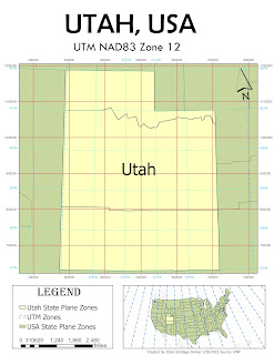
For our final map, we choose a state in the USA, and determined which projection to use; UTM vs State Plan.

I choose the state Utah because I have always wanted to go to Zion! I decided not to use the State Plane because there are three different ones that subdivide the state. Since state plane’s do not work here, I opted for UTM over Albers because we are looking at a relatively smaller area not close to the poles. I tried a couple of different UTM NAD83 Zones and landed on UTM NAD83 Zone 12. In this zone, Utah completely lies within one UTM Zone.

Comments

Utilizing ERDAS Imagine to Analyze Map Features

This week we learned how to utilize histograms and different bands to highlight different features in a map. On the following map that we worked on, dark bodies of water caused high peaks on the left of histograms while snow-peaked mountains were small blips on the far right. These simple distinctions help to quickly identify map features on a graph, that you can then utilize as a stepping stone to finding them on the image. I found it incredibly interesting how the different band layers highlighted different features on the map. Figure 1 below depicts three different features we found on the image. Figure 1: Distinct features found on an image using ERDAS Imagine. Feature 1: Large body of water. Feature 2: Snow-capped mountains transitioning to thick vegetation. Feature 3: Shallow turbulent body of water near urbanized land, transitioning to deep calm body of water.

Positional Accuracy: NSSDA

In this analysis, I compared the street and road intersect data collected for Alburquerque, NM by the City of Alburquerque and the application StreetMaps. I used an orthophoto base layer as the reference for this analysis, to compare and determine the accuracy of both the City and Streetmap layers using NSSDA procedures. The most difficult part of this analysis for me was how to determine what 20% per quadrant looks like. Because the reference map was divided into 208 quadrants, I had to determine how to subdivide all the quadrant's equality into 20%. After multiple trials and error, I decided to subdivide the entire area (208 sub-quadrants) into 4 equal-area subsections. In this way, I could do 5 random right intersection points per subsection or 20% per subsection. Map 1: City of Albuquerque city map data. Map 2: City of Alburquerque SteetMap data When selecting a random intersection to place the points within each quadrant, I choose a location that had data f...

Georeferencing, Editing, and Creating 3D Maps in ArcGIS Pro

During the last week of Intro to GIS, we learned how to utilize control points on an unreferenced map layer. This provided georeferenced points on the originally unreferenced map layer, placing it correctly on top of baselayers while using RSME as a guide to accuracy. Additionally, we edited map layers to add newer construction elements in the form of buildings and roads that were not previously on the map. Lastly, a LAS dataset was used in a Scene Map to create a 3D map of the main campus location of the University of West Florida. Below are the final maps for each of these steps. Figure 1: University of West Florida Main Campus Map. Ariel photographs georeferenced for accuracy, and new construction of gym building and Campus Lane edited into the map. A 330 and 660 ft buffer was also created around a protected eagles nest. Figure 2: 3D map of the Main Campus of the University of West Florida.

Piece of Eden GIS Blog

Search This Blog